Inferential Tests and Assumptions • gtstats

gtstats uses conservative, beginner-friendly defaults. Automatic selection can inspect the data, but it cannot determine whether observations are independent or whether the design and denominator answer the intended clinical question. Those decisions remain the analyst’s responsibility.

Quantify the magnitude separately

Use effect_size() when the question is how large a difference or association is. Its default output is deliberately smaller than compare_groups():

to_flextable(effect_size(mtcars, variable = mpg, group = am))

Measure	Contrast	Estimate	95% CI
Hedges' g	am: 0 − 1	-1.35	-2.18–-0.52
Direction: positive values indicate higher values or greater rank in 0; negative values indicate higher values or greater rank in 1.
95% CI: Approximate large-sample normal interval.

The automatic measure follows the comparison structure:

two continuous groups: Hedges’ g, with a confidence interval;
two-group rank comparison: rank-biserial correlation;
more than two continuous groups: omega-squared;
multi-group rank comparison: epsilon-squared;
categorical association: Cramer’s V.

For a two-group effect, the Contrast column explicitly names the grouping variable and uses its displayed order: first group minus second group. Positive and negative standardized or rank effects therefore have an unambiguous direction. Cramer’s V and omnibus measures describe association or overall variation and have no direction. Interval method information is retained in the notes; Hedges’ g intervals are labelled as approximate large-sample intervals.

An explicit method remains available when the scientific question requires it:

to_flextable(effect_size(
  mtcars,
  variable = mpg,
  group = am,
  method = "rank_biserial"
))

Measure	Contrast	Estimate	95% CI
Rank-biserial correlation	am: 0 − 1	-0.66	—
Direction: positive values indicate higher values or greater rank in 0; negative values indicate higher values or greater rank in 1.
A confidence interval is not currently available for Rank-biserial correlation.

Generic magnitude labels are excluded by default. Set interpretation = TRUE only when a conventional teaching label is useful; the table then states that this is not a threshold for clinical importance. For risk ratios, odds ratios, and risk differences, use crosstabs() so that the exposure and event direction remain explicit.

Default selection policy

compare_groups(test = "auto") follows these fixed rules. The selected test is never hidden: it is printed in the result and recorded with its rule and inputs in $method, $diagnostics, and $notes.

Comparison	What auto checks	Test selected
Continuous, two independent groups	Marked skewness within each group; `var_equal`	Welch t-test by default; Student’s t-test when `var_equal = TRUE`; Wilcoxon rank-sum only if one or more groups have marked skewness
Continuous, three or more independent groups	Marked skewness within each group; `var_equal`	Welch ANOVA by default; classical ANOVA when `var_equal = TRUE`; Kruskal-Wallis if one or more groups have marked skewness
Continuous, paired (two occasions)	Marked skewness of within-pair differences	Paired t-test if not flagged; Wilcoxon signed-rank if flagged
Continuous, paired (3+ occasions)	Marked skewness at each occasion	Repeated-measures ANOVA with Greenhouse-Geisser-corrected degrees of freedom if not flagged; Friedman test if flagged
Ordinal, independent	Expected cell counts	Pearson chi-square when no expected count is below 1 and no more than 20% are below 5; Fisher’s exact otherwise
Ordinal, paired	Outcome is ordered	Wilcoxon signed-rank (two occasions) or Friedman (3+ occasions)
Binary or nominal categorical, independent	Expected cell counts	Pearson chi-square when no expected count is below 1 and no more than 20% are below 5; Fisher’s exact otherwise
Binary, paired	Paired design and binary outcome	McNemar test (two occasions) or Cochran’s Q test (3+ occasions)

The continuous-variable switch means marked absolute sample skewness (default cut-off 1), not any asymmetry and not a normality-test p-value. Shapiro-Wilk is supporting information only and does not alone switch the test. add_p() uses the same rules.

Ordinal values: make the meaning explicit

compare_groups() retains an ordered factor’s ordinal classification, but for an independent Table 1 comparison it uses chi-square/Fisher to compare the distribution of all levels. Request test = "wilcox" or test = "kruskal" if the clinical question is specifically about the ordered ranks. A numeric variable with a few values (for example 0, 1, 2, 3 visits or cancer stages coded 1–4) is deliberately treated as a categorical/count-coded variable unless its order is explicitly declared. This avoids silently treating a clinical code as a numerical scale. Convert a true ordered variable before comparing it:

data$stage <- ordered(data$stage, levels = c(1, 2, 3, 4))
compare_groups(data, variable = stage, group = arm) # categorical distribution
compare_groups(data, variable = stage, group = arm, test = "wilcox") # rank shift

describe_data() makes this distinction visible: explicit ordered factors are shown as ordinal; small integer-coded variables receive a possible ordinal/count-coded flag for review against the data dictionary. It does not change the analysis type automatically.

Other automatic defaults are:

Question	Default
Estimate one proportion	Exact binomial confidence interval
Correlate two continuous variables	Pearson for approximately symmetric variables; otherwise Spearman
Estimate an event rate	Exact Poisson confidence interval

Proportions are estimates, not automatically tests

proportion_stats() estimates a proportion and Wilson score confidence interval. It does not test whether groups differ.

to_flextable(proportion_stats(mtcars, var = vs, by = am))

	1		0
Event	n (%)	95% CI	n (%)	95% CI
1	7 (53.8%)	29.1–76.8%	7 (36.8%)	19.1–59.0%
Selected event: vs = 1. Estimates use Wilson score 95% confidence intervals.
This function estimates a proportion; it does not test differences between groups.
The denominator must define the population at risk, and observations should be independent.

To compare categorical distributions, use compare_groups(), add_p(), or crosstabs().

to_flextable(compare_groups(mtcars, variable = vs, group = am))

Variable	Level	0 N = 19	1 N = 13	p-value
vs	0	12 (63.16%)	6 (46.15%)	0.56
	1	7 (36.84%)	7 (53.85%)
The analysis assumes independent observations; study design must confirm this.
Automatic selection used distribution guidance or design/cell-count rules. Rule applied: Independent categorical outcome; expected cell count guidance was met (no expected count below 1 and no more than 20% below 5); selected Pearson chi-square test.
Chi-square requires mutually exclusive categories and adequate expected cell counts.
Minimum expected cell count was 5.69; Fisher's exact test is selected automatically when an expected count is below 1 or more than 20% are below 5.

to_flextable(crosstabs(mtcars, row = am, col = vs))

am	0	1	Total
0	12 66.67%	7 50.00%	19 59.38%
1	6 33.33%	7 50.00%	13 40.62%
Total	18 100.00%	14 100.00%	32 100.00%
Cells are n (column %). Chi-square test with Yates correction, p = 0.556. Cramer's V = 0.17.
RR 1.46 (0.67–3.17); OR 2.00 (0.48–8.40); RD 17.00 pp (-16.15–45.98 pp)
Exposure: am; exposed = 1, unexposed = 0. Event: vs = 1. Complete observations: N = 32.

In automatic mode, expected cell counts are calculated. Fisher’s exact test is selected when an expected count is below 1 or more than 20% of expected cells are below 5; otherwise chi-square is used. Larger sparse tables use Fisher’s test with a Monte Carlo p-value. Returned objects expose the expected counts and the minimum expected count.

The analyst must still confirm:

observations are independent;
each observation contributes to one cell;
categories are mutually exclusive;
row and column levels have been defined in the intended direction.

For paired binary observations, supply an identifier and use McNemar’s test:

to_flextable(compare_groups(
  paired_data,
  variable = symptom_present,
  group = visit,
  paired = TRUE,
  id = id
))

Variable	Level	Baseline N = 90	Follow-up N = 90	p-value
Symptom present	No	38 (42.22%)	51 (56.67%)	0.09
	Yes	52 (57.78%)	39 (43.33%)
Analysis used 90 complete, uniquely matched binary pairs; 0 participants were excluded because a complete pair was not available.
Automatic selection used distribution guidance or design/cell-count rules. Rule applied: Paired binary outcome: selected McNemar test.
McNemar's test requires correctly matched binary pairs.

Continuous outcomes

Welch’s t-test is the two-group parametric default because it does not require equal variances. Welch ANOVA is the corresponding default for three or more groups. When equal variances are justified in a prespecified analysis plan, var_equal = TRUE changes the non-skewed independent automatic route to Student’s t-test or classical ANOVA. It does not run, infer, or prove an equal-variance hypothesis test.

Use assess_variance() to make the observed group spread visible before interpreting a comparison. It reports SDs, variances, and largest/smallest spread ratios and displays the median-centred Levene test by default. Bartlett is available as optional supporting information. These tests are never gatekeepers and do not change the automatic choice.

to_flextable(assess_variance(mtcars, vars = mpg, by = am))

Variable	1	0	Observed SD ratio	Observed variance ratio	Levene p	Interpretation
mpg	n = 13; SD = 6.17; variance = 38.03	n = 19; SD = 3.83; variance = 14.70	1.61	2.59	0.050	Levene suggests different spreads; interpret this with the study design.
SD and variance ratios are the largest group value divided by the smallest group value. They describe observed spread; they are not pass/fail tests.
For independent groups, Welch t-tests and Welch ANOVA do not require equal variances. `assess_variance()` does not select an inferential test and does not assess pairing or repeated-measures sphericity.
The displayed Levene test is median-centred (Brown-Forsythe). It is supporting information only: its p-value neither proves equal variances nor selects an inferential test.
Interpret spread alongside sample size, distributional shape, outliers, missingness, and the study design.

to_flextable(assess_variance(mtcars, vars = mpg, by = am, test = "none"))

Variable	1	0	Observed SD ratio	Observed variance ratio	Interpretation
mpg	n = 13; SD = 6.17; variance = 38.03	n = 19; SD = 3.83; variance = 14.70	1.61	2.59	Observed SD ratio shown; interpret it with the study design.
SD and variance ratios are the largest group value divided by the smallest group value. They describe observed spread; they are not pass/fail tests.
For independent groups, Welch t-tests and Welch ANOVA do not require equal variances. `assess_variance()` does not select an inferential test and does not assess pairing or repeated-measures sphericity.
Interpret spread alongside sample size, distributional shape, outliers, missingness, and the study design.

to_flextable(assess_variance(mtcars, vars = mpg, by = am, test = "bartlett"))

Variable	1	0	Observed SD ratio	Observed variance ratio	Bartlett p	Interpretation
mpg	n = 13; SD = 6.17; variance = 38.03	n = 19; SD = 3.83; variance = 14.70	1.61	2.59	0.072	Bartlett's test found no clear evidence of different spreads; this does not prove equal variances.
SD and variance ratios are the largest group value divided by the smallest group value. They describe observed spread; they are not pass/fail tests.
For independent groups, Welch t-tests and Welch ANOVA do not require equal variances. `assess_variance()` does not select an inferential test and does not assess pairing or repeated-measures sphericity.
Bartlett's test is supporting information only: it assumes normal group distributions, and its p-value neither proves equal variances nor selects an inferential test.
Interpret spread alongside sample size, distributional shape, outliers, missingness, and the study design.

The same observed-spread diagnostic is retained in an independent continuous compare_groups() result. It is descriptive context, not a test-selection rule: Welch t-tests and Welch ANOVA do not require equal variances. The value of var_equal is a transparent user choice, not a data-driven variance test.

to_flextable(compare_groups(
  mtcars,
  variable = mpg,
  group = am,
  test = "auto"
))

Variable	0 N = 19	1 N = 13	Mean difference (95% CI)	p-value
mpg	17.15 (3.83)	24.39 (6.17)	-7.24 (-11.28 to -3.21)	<0.01
The analysis assumes independent observations; study design must confirm this.
Automatic selection used distribution guidance or design/cell-count rules. Rule applied: Two-group continuous outcome: no skewness flag; `var_equal = FALSE`; selected Welch t-test, the conservative default that does not require equal variances.
Check within-group distributions for influential outliers and substantial departures from normality, particularly in small samples.


to_flextable(compare_groups(mtcars, variable = mpg, group = cyl))

Variable	4 N = 11	6 N = 7	8 N = 14	p-value
mpg	26.66 (4.51)	19.74 (1.45)	15.10 (2.56)	<0.01
The analysis assumes independent observations; study design must confirm this.
Automatic selection used distribution guidance or design/cell-count rules. Rule applied: Multi-group continuous outcome: no skewness flag; `var_equal = FALSE`; selected Welch ANOVA, the conservative default that does not require equal variances.
Welch ANOVA allows unequal variances; check residual shape and influential outliers.

to_flextable(compare_groups(mtcars, variable = mpg, group = cyl, test = "anova"))

Variable	4 N = 11	6 N = 7	8 N = 14	p-value
mpg	26.66 (4.51)	19.74 (1.45)	15.10 (2.56)	<0.01
The analysis assumes independent observations; study design must confirm this.
Classical ANOVA assumes approximately normal residuals and similar group variances.

Distribution guidance primarily uses skewness. Shapiro-Wilk results are supporting information and are not used alone to select a test. Analysts should also inspect outliers and plots. To see the exact automatic decision for one analysis, inspect the saved result:

result <- compare_groups(mtcars, variable = mpg, group = am)
result$method$selection_rule
#> [1] "Two-group continuous outcome: no skewness flag; `var_equal = FALSE`; selected Welch t-test, the conservative default that does not require equal variances."
result$method$selection_inputs
#> $distribution_guidance
#> [1] "Approximately symmetric; Approximately symmetric"
#> 
#> $skewness_flagged
#> [1] FALSE
#> 
#> $groups
#> [1] 2
#> 
#> $paired
#> [1] FALSE
#> 
#> $var_equal
#> [1] FALSE
#> 
#> $variance_assumption_source
#> [1] "User-specified; not inferred from a variance hypothesis test"
#> 
#> $observed_group_spread
#> $observed_group_spread$group_spread
#> # A tibble: 2 × 4
#>   group     n    sd variance
#>   <chr> <int> <dbl>    <dbl>
#> 1 0        19  3.83     14.7
#> 2 1        13  6.17     38.0
#> 
#> $observed_group_spread$sd_ratio
#> [1] 1.608388
#> 
#> $observed_group_spread$variance_ratio
#> [1] 2.586911
diagnostics_stats(result)

Variable	Check	Result	Observed value	Reference	Interpretation
Diagnostics
mpg	Comparison design	independent	Independent observations	Defined by the study design	Independent comparison; confirm independence from the study design.
mpg	Variance assumption	welch default	var_equal = FALSE	User-specified analytical assumption	Welch is the conservative default and does not require equal variances. No variance hypothesis test was used.
mpg	Automatic test selection	Welch t-test	Approximately symmetric; Approximately symmetric	No marked group-level skewness flag for parametric default	Two-group continuous outcome: no skewness flag; `var_equal = FALSE`; selected Welch t-test, the conservative default that does not require equal variances.
mpg	Distribution guidance	parametric reasonable	Approximately symmetric; Approximately symmetric	Marked absolute skewness guidance; Shapiro-Wilk is supporting information only	Assessment applied within each group.
mpg	Observed group spread	descriptive context	0 (n = 19): SD 3.83; variance 14.70; 1 (n = 13): SD 6.17; variance 38.03; SD ratio = 1.61; variance ratio = 2.59	Descriptive diagnostic; no pass/fail threshold	Observed spread is descriptive only; no Levene, Bartlett, or F test was performed. `var_equal = FALSE` retains Welch methods as the conservative parametric auto default.

Wilcoxon rank-sum and Kruskal-Wallis tests compare ranks. Interpreting them specifically as median comparisons requires broadly similar distribution shapes across groups.

For paired continuous analyses, distribution guidance is applied to the within-pair differences rather than each measurement occasion separately.

Summary-table p-values

add_p() uses the same automatic selection policy as compare_groups(). Distribution guidance is enabled by default.

summary_table(mtcars, by = am, include = c(mpg, wt, vs), overall = TRUE) |>
  add_p() |>
  to_flextable()

Characteristic	Overall N = 32	1 N = 13	0 N = 19	p-value
mpg	20.1 (6.0)	24.4 (6.2)	17.1 (3.8)	0.001ᵃ
wt	3.2 (1.0)	2.4 (0.6)	3.8 (0.8)	<0.001ᵃ
vs				0.556ᵇ
0	18 (56.2%)	6 (46.2%)	12 (63.2%)
1	14 (43.8%)	7 (53.8%)	7 (36.8%)
Continuous data are mean (SD). Categorical data are n (%).
ᵃ Welch t-test; ᵇ Chi-square test

Tests can be prespecified per variable:

summary_table(mtcars, by = am, include = c(mpg, wt, vs)) |>
  add_p(
    test = c(
      mpg = "welch_t",
      wt = "wilcox",
      vs = "fisher"
    ),
    distribution_check = FALSE
  ) |>
  to_flextable()

Characteristic	1 N = 13	0 N = 19	p-value
mpg	24.4 (6.2)	17.1 (3.8)	0.001ᵃ
wt	2.4 (0.6)	3.8 (0.8)	<0.001ᵇ
vs			0.473ᶜ
0	6 (46.2%)	12 (63.2%)
1	7 (53.8%)	7 (36.8%)
Continuous data are mean (SD). Categorical data are n (%).
ᵃ Welch t-test; ᵇ Wilcoxon rank-sum test; ᶜ Fisher's exact test

To use the equal-variance parametric route deliberately:

to_flextable(compare_groups(trial_data, change_score, group = arm, var_equal = TRUE))

Variable	Treatment A N = 60	Treatment B N = 60	Usual care N = 60	p-value
Change in clinical score	4.20 (5.69)	6.47 (7.34)	-0.37 (6.24)	<0.01
The analysis assumes independent observations; study design must confirm this.
Automatic selection used distribution guidance or design/cell-count rules. Rule applied: Multi-group continuous outcome: no skewness flag; equal variance was user-specified (`var_equal = TRUE`); selected classical one-way ANOVA. No variance hypothesis test was used.
Classical ANOVA assumes approximately normal residuals and similar group variances.

The table footnote records tests used and reminds readers that independence must be confirmed from the study design.

Correlation

Automatic correlation selection uses marginal distribution shape, but this cannot confirm the shape of the relationship. Inspect a scatterplot:

Pearson requires an approximately linear relationship.
Spearman requires a monotonic relationship.

With method = "auto", correlation() uses Pearson only when both marginal absolute sample skewness values are below 1; otherwise it uses Spearman. This is a transparent default, not proof that the relationship is linear or monotonic. Inspect plot_correlation() before reporting the coefficient. diagnostics_stats() records the two skewness values, selected rule, and the number of complete finite pairs used. - Both require independent observation pairs without dominating influential observations.

For exploratory work with several continuous variables, supply vars instead of x and y. One method is deliberately used throughout the matrix, avoiding a confusing mixture of Pearson and Spearman coefficients. Each pair may have a different denominator when values are missing, so inspect $summary before reporting selected results.

matrix_result <- correlation(
  mtcars,
  vars = c(mpg, disp, hp, wt),
  display = "estimate_p",
  adjust = "holm"
)

to_flextable(matrix_result)

Variable	mpg	disp	hp	wt
mpg	1.00
disp	-0.85 p = <0.01	1.00
hp	-0.78 p = <0.01	0.79 p = <0.01	1.00
wt	-0.87 p = <0.01	0.89 p = <0.01	0.66 p = <0.01	1.00
All selected variables had absolute sample skewness below 1; Pearson was used throughout.
Each coefficient uses pairwise complete finite observations; sample sizes can differ between pairs.
Matrix p-values use the holm multiplicity adjustment.
Correlation does not imply causation. Inspect relevant pairwise plots before interpretation.

plot_correlation(matrix_result)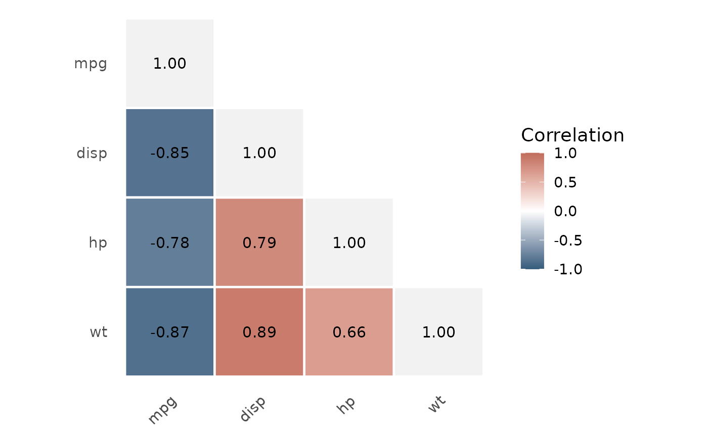

The heatmap shows direction and magnitude, not importance or causality. Multiplicity adjustment is available for exploratory p-values, but a matrix does not replace a prespecified research question.

Rates

rate_stats() estimates rates with exact Poisson confidence intervals. Confirm that:

events are valid counts;
person-time or exposure time is positive and correctly accumulated;
observations or event processes are suitably independent;
a Poisson process is a reasonable approximation.

Counts per 100 people at a single time point are proportions, not incidence rates, unless genuine observation time is represented.

Inspect what was checked

Inferential objects retain transparent metadata:

result <- compare_groups(mtcars, variable = vs, group = am)

result$inferential
#> # A tibble: 1 × 27
#>   outcome label outcome_type group group_levels test_requested test_used  paired
#>   <chr>   <chr> <chr>        <chr>        <int> <chr>          <chr>      <lgl> 
#> 1 vs      vs    binary       am               2 auto           Chi-squar… FALSE 
#> # ℹ 19 more variables: statistic <dbl>, df <int>, p_value <dbl>,
#> #   estimate <dbl>, estimate_type <chr>, conf_low <dbl>, conf_high <dbl>,
#> #   conf_level <dbl>, effect_size <dbl>, effect_size_type <chr>,
#> #   effect_size_interpretation <chr>, method_detail <chr>,
#> #   reason_for_test <chr>, interpretation <chr>, notes <chr>,
#> #   effect_size_symbol <chr>, effect_conf_low <dbl>, effect_conf_high <dbl>,
#> #   effect_interval_method <chr>
result$method
#> $outcome_type
#> [1] "binary"
#> 
#> $group_type
#> [1] "binary"
#> 
#> $test_requested
#> [1] "auto"
#> 
#> $test_selected
#> [1] "Chi-square test"
#> 
#> $variance_assumption
#> $variance_assumption$value
#> [1] FALSE
#> 
#> $variance_assumption$source
#> [1] "User-specified; not inferred from a variance hypothesis test"
#> 
#> $variance_assumption$applies
#> [1] FALSE
#> 
#> 
#> $selection_rule
#> [1] "Independent categorical outcome; expected cell count guidance was met (no expected count below 1 and no more than 20% below 5); selected Pearson chi-square test."
#> 
#> $selection_inputs
#> $selection_inputs$groups
#> [1] 2
#> 
#> $selection_inputs$outcome_type
#> [1] "binary"
#> 
#> $selection_inputs$minimum_expected_count
#> [1] 5.6875
#> 
#> $selection_inputs$expected_count_threshold
#> [1] "No expected count < 1 and <=20% below 5"
#> 
#> $selection_inputs$expected_count_screen
#> $selection_inputs$expected_count_screen$sparse
#> [1] FALSE
#> 
#> $selection_inputs$expected_count_screen$any_below_1
#> [1] FALSE
#> 
#> $selection_inputs$expected_count_screen$proportion_below_5
#> [1] 0
#> 
#> $selection_inputs$expected_count_screen$n_below_5
#> [1] 0
#> 
#> $selection_inputs$expected_count_screen$n_cells
#> [1] 4
#> 
#> 
#> 
#> $expected_counts
#>             outcome_clean
#> group_factor       0      1
#>            0 10.6875 8.3125
#>            1  7.3125 5.6875
#> 
#> $expected_count_screen
#> $expected_count_screen$sparse
#> [1] FALSE
#> 
#> $expected_count_screen$any_below_1
#> [1] FALSE
#> 
#> $expected_count_screen$proportion_below_5
#> [1] 0
#> 
#> $expected_count_screen$n_below_5
#> [1] 0
#> 
#> $expected_count_screen$n_cells
#> [1] 4
#> 
#> 
#> $fisher_simulation
#> NULL
result$assumptions
#> # A tibble: 3 × 4
#>   assumption                    status     result       detail                  
#>   <chr>                         <chr>      <chr>        <chr>                   
#> 1 Independent observations      user_check not_checked  Confirm from the study …
#> 2 Mutually exclusive categories user_check not_checked  Confirm that every obse…
#> 3 Adequate expected cell counts checked    guidance_met Automatic selection use…
result$diagnostics
#> # A tibble: 4 × 5
#>   check                    result          value                threshold detail
#>   <chr>                    <chr>           <chr>                <chr>     <chr> 
#> 1 Comparison design        independent     Independent observa… Defined … Indep…
#> 2 Variance assumption      not_applicable  var_equal = FALSE    Applies … `var_…
#> 3 Automatic test selection Chi-square test 5.69                 No expec… Indep…
#> 4 Expected cell counts     guidance_met    5.69                 No expec… Fishe…
result$denominators
#> # A tibble: 2 × 9
#>   variable level group  n_total n_nonmissing n_missing numerator denominator
#>   <chr>    <chr> <chr>    <int>        <int>     <int>     <dbl>       <dbl>
#> 1 vs       NA    am = 1      13           13         0        NA          13
#> 2 vs       NA    am = 0      19           19         0        NA          19
#> # ℹ 1 more variable: rule <chr>
result$notes
#> [1] "The analysis assumes independent observations; study design must confirm this."                                                                                                                                                                            
#> [2] "Automatic selection used distribution guidance or design/cell-count rules. Rule applied: Independent categorical outcome; expected cell count guidance was met (no expected count below 1 and no more than 20% below 5); selected Pearson chi-square test."
#> [3] "Chi-square requires mutually exclusive categories and adequate expected cell counts."                                                                                                                                                                      
#> [4] "Minimum expected cell count was 5.69; Fisher's exact test is selected automatically when an expected count is below 1 or more than 20% are below 5."

$inferential records the selected test and reason. $method contains detected variable types and method metadata. $assumptions distinguishes automatic checks from requirements that must be confirmed from the study design. $diagnostics records check results, values, thresholds and interpretation. $denominators records total, non-missing and missing observations together with the numerator, denominator, group and rule used. $notes remains a short human-readable explanation.

Use the inspection helpers for a consistent tibble or formatted table:

assumptions_stats(result)

Variable	Check before reporting	Action	Details
Checks before reporting
vs	Independent observations	Confirm from study design	Confirm from the study design that each observation contributes independently.
vs	Mutually exclusive categories	Confirm from study design	Confirm that every observation contributes to one category per variable.
vs	Adequate expected cell counts	Checked automatically	Automatic selection uses Fisher's exact test when any expected count is below 1 or more than 20% are below 5.

diagnostics_stats(result)

Variable	Check	Result	Observed value	Reference	Interpretation
Diagnostics
vs	Comparison design	independent	Independent observations	Defined by the study design	Independent comparison; confirm independence from the study design.
vs	Variance assumption	not applicable	var_equal = FALSE	Applies only to independent parametric continuous comparisons	`var_equal` does not alter paired, categorical, ordinal, or rank-based routes.
vs	Automatic test selection	Chi-square test	5.69	No expected count below 1 and no more than 20% below 5	Independent categorical outcome; expected cell count guidance was met (no expected count below 1 and no more than 20% below 5); selected Pearson chi-square test.
vs	Expected cell counts	guidance met	5.69	No expected count below 1 and no more than 20% below 5	Fisher's exact test is selected automatically when expected-count guidance is not met.

denominators_stats(result)

Variable	Level	Group	Eligible observations	Used in analysis	Missing / excluded	Numerator	Denominator	Rule
Denominator audit
vs	NA	am = 1	13	13	0	NA	13	Non-missing outcome observations within group
vs	NA	am = 0	19	19	0	NA	19	Non-missing outcome observations within group


denominators_stats(result, format = "tibble")
#> # A tibble: 2 × 9
#>   Variable Level Group  `Eligible observations` `Used in analysis`
#>   <chr>    <chr> <chr>                    <int>              <int>
#> 1 vs       NA    am = 1                      13                 13
#> 2 vs       NA    am = 0                      19                 19
#> # ℹ 4 more variables: `Missing / excluded` <int>, Numerator <dbl>,
#> #   Denominator <dbl>, Rule <chr>

These audit helpers are intentionally separate from the publication table:

assumptions_stats() records what the method assumes, including items that require design or clinical judgement rather than a software check.
diagnostics_stats() shows numerical checks and automatic decisions in plain language; use view = "audit" for the underlying technical codes.
denominators_stats() shows the analysed observations, missing values, numerators and denominators behind reported percentages, rates and risks; view = "audit" returns the underlying field names.

Use them to review an analysis before reporting it; they are not normally included in a manuscript table.